How To Change A Column To A Row In Excel

Lesson 6: Modifying Columns, Rows, and Cells

/en/excel/cell-nuts/content/

Introduction

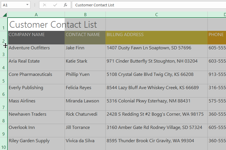
By default, every row and column of a new workbook is set to the aforementioned height and width. Excel allows y'all to modify column width and row height in different ways, including wrapping text and merging cells.

Optional: Download our practice workbook.

Watch the video below to learn more than about modifying columns, rows, and cells.

To modify column width:

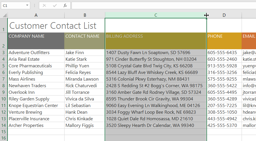
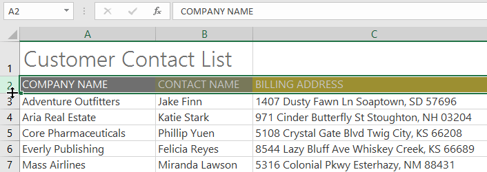
In our instance below, column C is too narrow to display all of the content in these cells. Nosotros can brand all of this content visible past changing the width of column C.

Position the mouse over the column line in the cavalcade heading so the cursor becomes a double arrow.
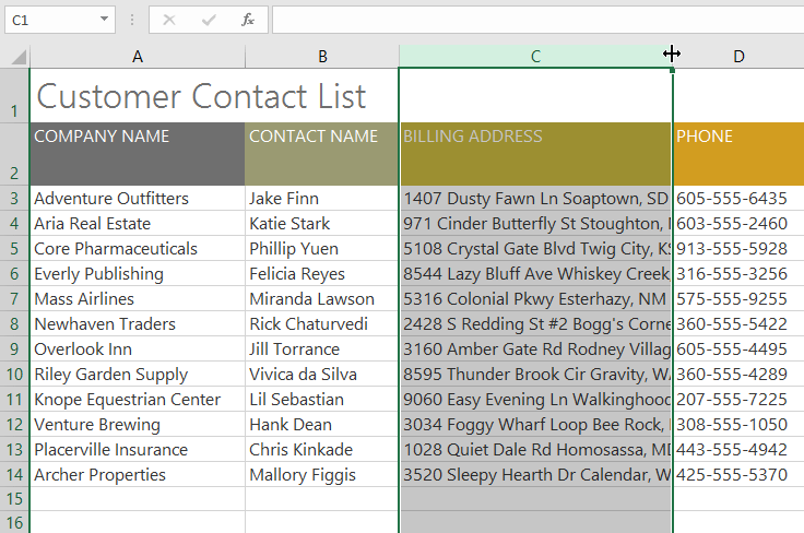
Click and drag the mouse to increase or decrease the column width.
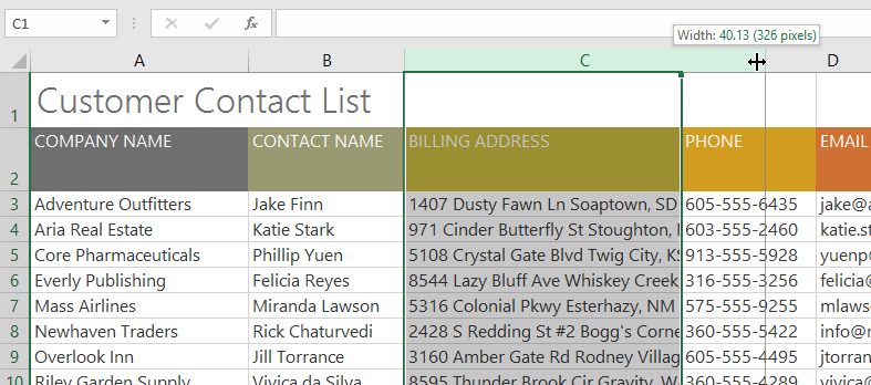
Release the mouse. The column width volition exist changed.

With numerical data, the cell will brandish pound signs (#######) if the column is as well narrow. Simply increment the column width to brand the data visible.

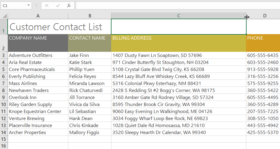
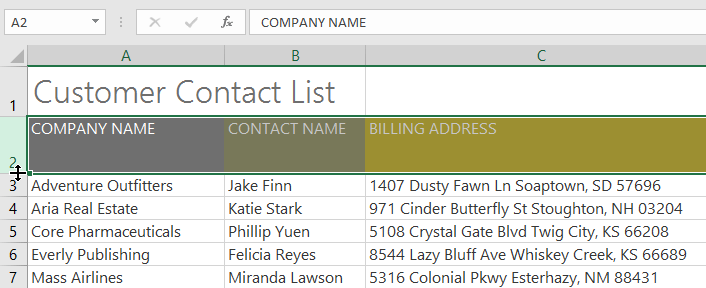
To AutoFit column width:

The AutoFit characteristic volition allow you to set a column'southward width to fit its content automatically.

Position the mouse over the cavalcade line in the column heading so the cursor becomes a double arrow.
Double-click the mouse. The column width will be changed automatically to fit the content.

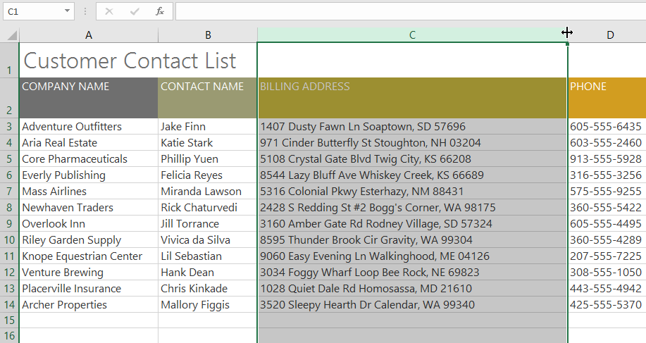
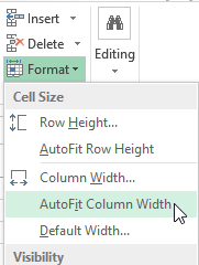
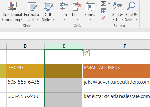
You can also AutoFit the width for several columns at the same fourth dimension. Merely select the columns you want to AutoFit, then select the AutoFit Column Width control from the Format drop-downwards menu on the Home tab. This method tin also be used for row height.

autofitting column width for multiple columns

To modify row peak:

Position the cursor over the row line so the cursor becomes a double arrow.
Click and drag the mouse to increase or decrease the row peak.
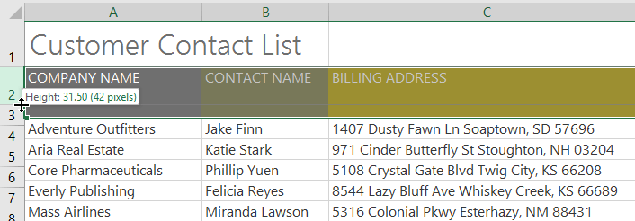
Release the mouse. The top of the selected row will be inverse.

To modify all rows or columns:

Instead of resizing rows and columns individually, you can alter the height and width of every row and cavalcade at the same time. This method allows you to set a uniform size for every row and column in your worksheet. In our example, we will set up a uniform row elevation.

Locate and click the Select All button just below the name box to select every cell in the worksheet.
Position the mouse over a row line so the cursor becomes a double arrow.
Click and elevate the mouse to increase or decrease the row height, then release the mouse when you are satisfied. The row height will be changed for the entire worksheet.

Inserting, deleting, moving, and hiding

Subsequently yous've been working with a workbook for a while, y'all may notice that you desire to insert new columns or rows, delete certain rows or columns, move them to a different location in the worksheet, or even hide them.

To insert rows:

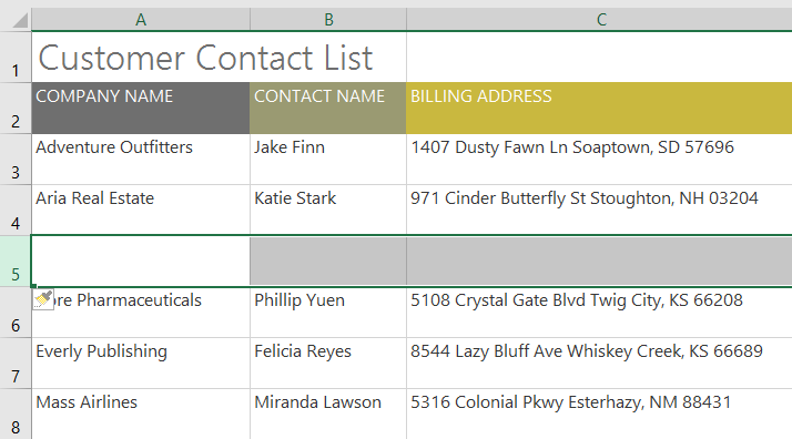
Select the row heading below where you lot want the new row to appear. In this example, we want to insert a row between rows 4 and 5, so we'll select row 5.
Click the Insert command on the Home tab.
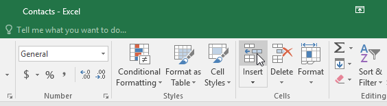
The new row will appear above the selected row.

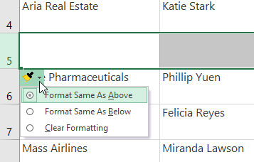
When inserting new rows, columns, or cells, yous will see a paintbrush icon adjacent to the inserted cells. This button allows you to choose how Excel formats these cells. By default, Excel formats inserted rows with the same formatting as the cells in the row above. To access additional options, hover your mouse over the icon, then click the drop-down pointer.

choosing more insert formatting options

To insert columns:

Select the cavalcade heading to the right of where you want the new column to appear. For example, if you want to insert a column betwixt columns D and E, select column Eastward.
Click the Insert command on the Dwelling tab.
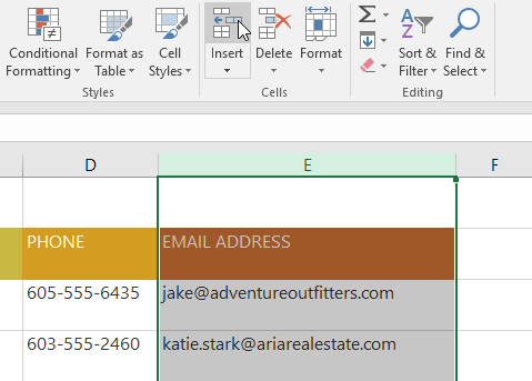
The new column volition announced to the left of the selected column.

When inserting rows and columns, make sure to select the entire row or cavalcade by clicking the heading. If you select only a cell in the row or column, the Insert command will only insert a new cell.

To delete a row or cavalcade:

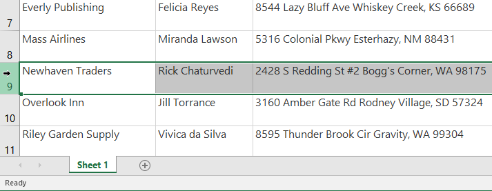
Information technology'southward easy to delete a row or column that you no longer need. In our example we'll delete a row, merely you can delete a column the same way.

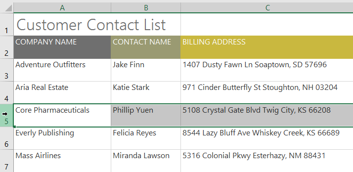
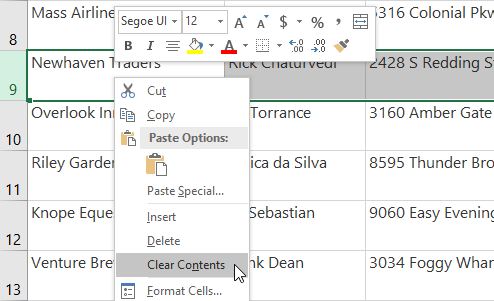
Select the row yous want to delete. In our case, we'll select row 9.
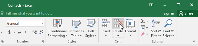
Click the Delete command on the Home tab.
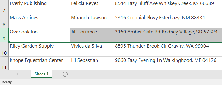
The selected row volition be deleted, and those effectually it will shift. In our case, row 10 has moved upwards, then it'south now row ix.

It'south of import to understand the difference between deleting a row or column and simply immigration its contents. If you want to remove the content from a row or column without causing others to shift, correct-click a heading, and so select Articulate Contents from the driblet-downwards menu.

clearing the contents of a row instead of deleting

To motility a row or cavalcade:

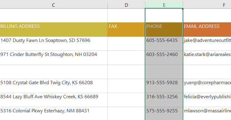
Sometimes you may desire to move a column or row to rearrange the content of your worksheet. In our example we'll motion a column, but y'all can movement a row in the same way.

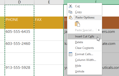
Select the desired column heading for the cavalcade you want to move.
Click the Cut command on the Home tab, or printing Ctrl+10 on your keyboard.
Select the column heading to the right of where y'all desire to motility the cavalcade. For example, if you want to move a cavalcade between columns Eastward and F, select column F.
Click the Insert command on the Domicile tab, and then select Insert Cut Cells from the drop-down carte.
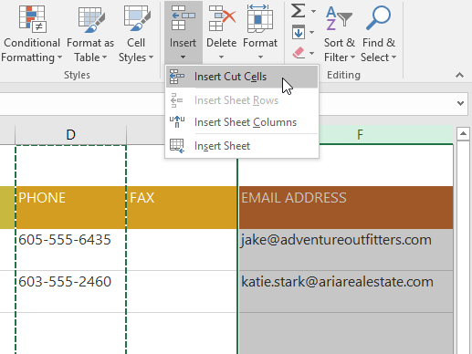
The column will be moved to the selected location, and the columns around it will shift.

You can as well access the Cut and Insert commands by right-clicking the mouse and selecting the desired commands from the drop-down menu.

accessing commands from the right-click menu

To hide and unhide a row or column:

At times, you may want to compare certain rows or columns without irresolute the organization of your worksheet. To do this, Excel allows you to hide rows and columns equally needed. In our instance we'll hide a few columns, just you tin hide rows in the same mode.

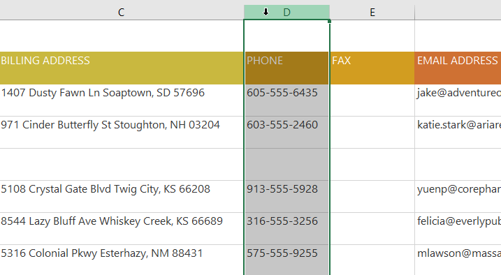
Select the columns you want to hide, correct-click the mouse, then select Hide from the formatting menu. In our example, we'll hibernate columns C, D, and East.
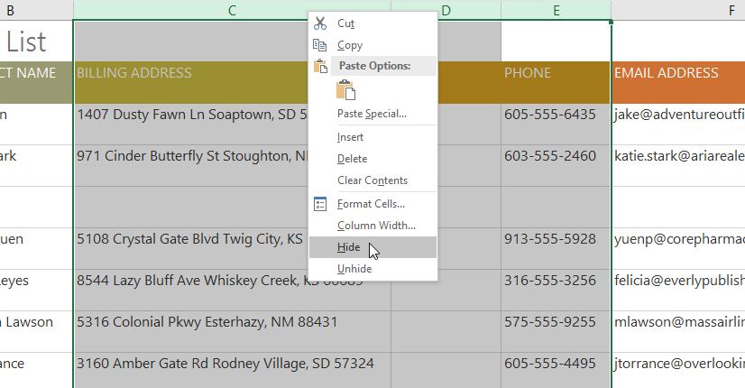
The columns will exist hidden. The green column line indicates the location of the hidden columns.
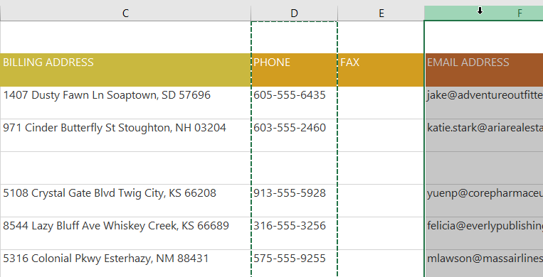
To unhide the columns, select the columns on both sides of the hidden columns. In our instance, nosotros'll select columns B and F. Then right-click the mouse and select Unhide from the formatting menu.
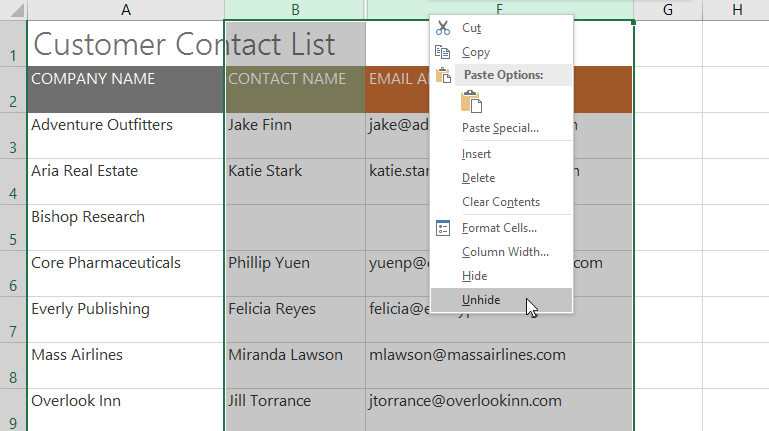
The subconscious columns will reappear.

Wrapping text and merging cells

Whenever you have too much cell content to be displayed in a single cell, you may determine to wrap the text or merge the cell rather than resize a column. Wrapping the text will automatically alter a cell's row height, allowing cell contents to exist displayed on multiple lines. Merging allows you to combine a cell with adjacent empty cells to create ane big cell.

To wrap text in cells:

Select the cells you want to wrap. In this example, we'll select the cells in column C.
Click the Wrap Text command on the Home tab.
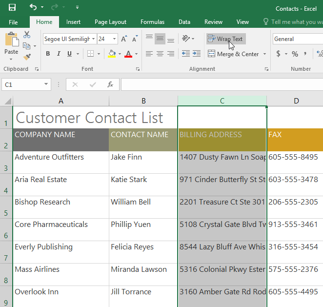
The text in the selected cells will be wrapped.

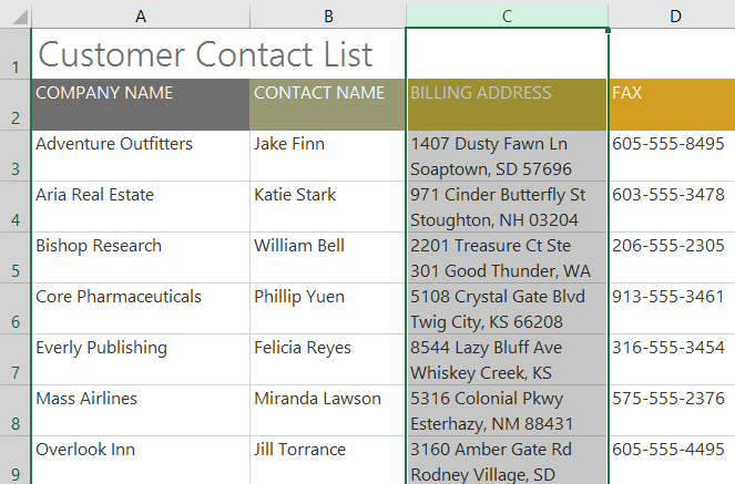
Click the Wrap Text command again to unwrap the text.

To merge cells using the Merge & Heart command:

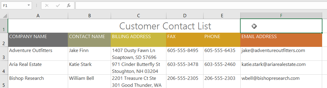
Select the cell range you want to merge. In our instance, we'll select A1:F1.
Click the Merge & Center command on the Home tab. In our example, we'll select the cell range A1:F1.
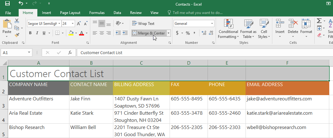
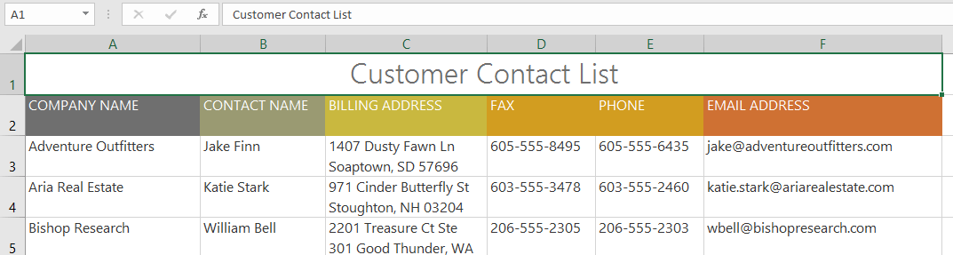
The selected cells volition be merged, and the text volition exist centered.

To access additional merge options:

If you lot click the driblet-down pointer next to the Merge & Center control on the Home tab, the Merge drop-down menu will appear.

other cell merge options

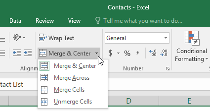
From here, you can choose to:

Merge & Center: This merges the selected cells into one cell and centers the text.
Merge Beyond: This merges the selected cells into larger cells while keeping each row split up.
Merge Cells: This merges the selected cells into one cell merely does not center the text.
Unmerge Cells: This unmerges selected cells.

Be careful when using this feature. If you merge multiple cells that all comprise data, Excel will go along just the contents of the upper-left cell and discard everything else.

Centering across selection

Merging can be useful for organizing your data, but it can likewise create problems afterwards. For example, it tin can be difficult to move, re-create, and paste content from merged cells. A good alternative to merging is to Center Beyond Selection , which creates a like effect without actually combining cells.

Spotter the video beneath to learn why you should use Middle Across Pick instead of merging cells.

To apply Middle Across Selection:

Select the desired cell range. In our example, nosotros'll select A1:F1. Note: If you lot already merged these cells, you should unmerge them before continuing to step 2.
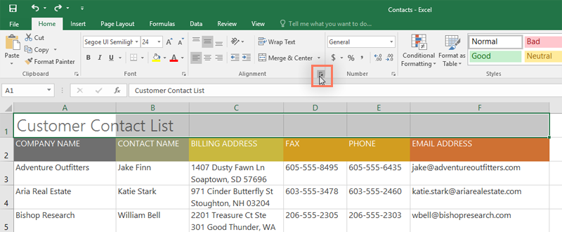
Click the pocket-size arrow in the lower-right corner of the Alignment group on the Home tab.
A dialog box will appear. Locate and select the Horizontal drop-downwardly bill of fare, select Heart Beyond Selection, then click OK.
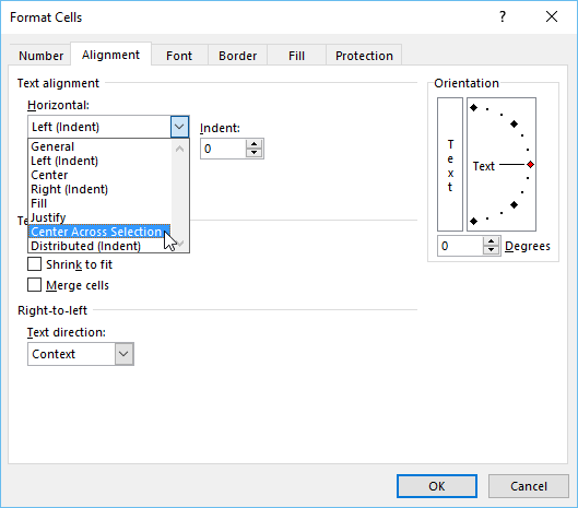
The content will be centered across the selected prison cell range. Every bit you can meet, this creates the same visual result as merging and centering, just it preserves each cell within A1:F1.

Claiming!

Open our practise workbook.
Autofit Column Width for the entire workbook.
Alter the row height for rows 3 to fourteen to 22.v (thirty pixels).
Delete row 10.
Insert a column to the left of cavalcade C. Type SECONDARY CONTACT in jail cell C2.
Make sure cell C2 is however selected and choose Wrap Text.
Merge and Center cells A1:F1.
Hide the Billing Accost and Phone columns.
When you're finished, your workbook should look something like this: